

Visualizing data is a great way to both derive insights and to validate the quality of a data set. There are a number of ways to draw plots in Python. Two of the popular libraries we use are:
- Matplotlib: a 2D plotting library that can create publication-quality figures in a variety of hardcopy formats
- Bokeh: an interactive visualization library for web browsers
Matplotlib
Matplotlib is a likely the most popular plotting library for python-based data analysis. Plots can be generated quickly and interactively. It fits naturally into the data analysis workflow for scientists and engineers, particularly when using Research and Development IDEs discussed in our earlier article on Different Ways of Running Python Code. The first round of plots can be created with a few simple function calls. This is great for deriving insights. However, going from the working visual to a publication-quality figure can take a significant chunk of code.
A figure generated using Matplotlib is initially interactive. Zooming, panning, saving and other basic interactions are supported. The figure can be saved in common image formats (PNG, JPEG, PDF, SVG). Once saved, however, the image is like any other image. It loses the interactive capability. Recreating the interactive figure requires executing the original script which created the matplotlib figure.
This fulfills the plotting needs for a significant portion of science and engineering work. There are two cases where Matplotlib is not useful:
- Saving an interactive figure that a colleague can visualize without executing the original script.
- Sharing the interactive figure via a web browser
The Bokeh library is able to fill this gap.
Bokeh
Bokeh is designed to create web browser visualizations that are both interactive and responsive. The library is built to support both small and large data sets as well as work with streaming datasets. This is great for embedding plots into web sites or data dashboards.
Plotting Example
The sample data we will work with comes from sensors aboard Unmanned Aerial Vehicles flown by researchers at the University of Minnesota. The complete data set is accessible from the University conservancy: Reference Position and Attitude together with Raw Sensor Data from Seven Small UAV Flights during 2011-12.
To simplify our example, we will access the data using a library supported by Organic Navigation named onavdata. This will let us load the flight data quickly. We will work with a flight from 2012 from an aircraft named THOR.
The Sample Data
The sample data can be loaded and the information available quickly explored:
import onavdata
df = onavdata.get_data('2012 UMN-UAV THOR75')
print(df.info())
Data columns (total 29 columns):
 #   Column                          Non-Null Count  Dtype
---  ------                          --------------  -----
 0   AccelX (m/s^2)                  23810 non-null  float64
 1   AccelY (m/s^2)                  23810 non-null  float64
 2   AccelZ (m/s^2)                  23810 non-null  float64
 3   AngleRateX (rad/s)              23810 non-null  float64
 4   AngleRateY (rad/s)              23810 non-null  float64
 5   AngleRateZ (rad/s)              23810 non-null  float64
 6   MagFieldX (G)                   23810 non-null  float64
 7   MagFieldY (G)                   23810 non-null  float64
 8   MagFieldZ (G)                   23810 non-null  float64
 9   AngleHeading (rad)              23810 non-null  float64
 10  AnglePitch (rad)                23810 non-null  float64
 11  AngleRoll (rad)                 23810 non-null  float64
 12  PosLat (deg)                    23810 non-null  float64
 13  PosLon (deg)                    23810 non-null  float64
 14  PosAlt (m)                      23810 non-null  float64
 15  GNSSPosLat (deg)                23710 non-null  float64
 16  GNSSPosLon (deg)                23710 non-null  float64
 17  GNSSPosAlt (m)                  23710 non-null  float64
 18  GNSSVelNorth (m/s)              23710 non-null  float64
 19  GNSSVelEast (m/s)               23710 non-null  float64
 20  GNSSVelDown (m/s)               23710 non-null  float64
 21  PitotAirSpeed (m/s)             23810 non-null  float64
 22  BaroAlt (m)                     23810 non-null  float64
 23  ModeAutopilot (1:human 2:auto)  23810 non-null  int64
 24  InputThrottle (0-1)             23810 non-null  float64
 25  InputElevator (0-1)             23810 non-null  float64
 26  InputRudder (0-1)               23810 non-null  float64
 27  InputAileronLeft (0-1)          23810 non-null  float64
 28  InputAileronRight (0-1)         23810 non-null  float64
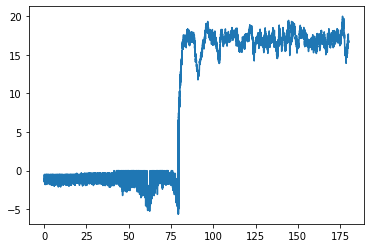
For this example we will visualize with the aircraft airspeed sensor PitotAirSpeed (m/s).
Basic Matplotlib Plot
#
# Load Data File & Peak at Entries
#
import onavdata
df = onavdata.get_data('2012 UMN-UAV THOR75')
df = df[df.index < 180] # Limit data to first 180 seconds

# Save time and airspeed into separate variables
t_sec = df.index
airspeed_mps = df['PitotAirSpeed (m/s)']

#
# Create a plot to visualize 2D-position and heading angle
#
from matplotlib import pyplot as plt
plt.plot(t_sec, airspeed_mps)
plt.show()
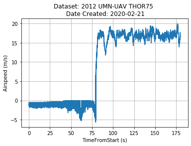
Publication Quality Matplotlib Plot
#
# Load Data File & Peak at Entries
#
import onavdata
df = onavdata.get_data('2012 UMN-UAV THOR75')
df = df[df.index < 180] # Limit data to first 180 seconds

# Save time and airspeed into separate variables
t_sec = df.index
airspeed_mps = df['PitotAirSpeed (m/s)']

#
# Create a plot to visualize 2D-position and heading angle
#
from matplotlib import pyplot as plt

plt.plot(t_sec, airspeed_mps)

plt.xlabel('TimeFromStart (s)')
plt.ylabel('Airspeed (m/s)')
plt.title('Dataset: 2012 UMN-UAV THOR75 \n Date Created: 2020-02-21')
plt.grid()

plt.show()
Basic Bokeh Plot
#
# Load Data File & Peak at Entries
#
import onavdata
df = onavdata.get_data('2012 UMN-UAV THOR75')
df = df[df.index < 180] # Limit data to first 180 seconds

# Save time and airspeed into separate variables
t_sec = df.index
airspeed_mps = df['PitotAirSpeed (m/s)']

#
# Create a plot to visualize 2D-position and heading angle
#
from bokeh.plotting import figure, output_file, save

# Set output html
output_file('bokeh_plot_01.html')
p = figure(plot_width=900,
           plot_height=200,
           x_axis_label='TimeFromStart (s)',
           y_axis_label='PitotAirSpeed (m/s)')
p.line(t_sec, airspeed_mps, line_width=2)
save(p)
Note that you can interactively work with the Bokeh plot by zooming in, panning, and saving the plot if needed.
Conclusion
This demonstrates two powerful libraries for visualizing data. Together, we have found that Matplotlib and Bokeh cover most use cases for scientists and engineers. Hopefully the above examples illstrates how to use either library and this article has helped you get started with using python for your own visualization needs.